Flex Attention and Triton, Supporting Long Context Training in SpecForge

Earlier this year, I had a post on how EAGLE3 speculative decoding works in SGLang. EAGLE3 has an advantage over MTP(Multi-Token Prediction) as MTP is usually trained together during the pre-training phase. However, EAGLE3 can be trained seperately. At LinkedIn, where we fine-tuned open source LLMs most of the time, EAGLE3 was a great fit for our use cases.

SGLang community has released a open source project named SpecForge, which is a framework for training speculative decoding draft models, particularly EAGLE3, to speed up inference of LLMs. We quickly adopted SpecForge into LinkedIn’s internal use cases such as LLM-as-a-Judge and Agentic LLMs. During the training, we encountered challenges to scale the training up in the long context scenarios. Especially for the agentic use cases, our training data can easily reach 16K or even 32K tokens in length. In this post, I will summarize how we used Flex Attention and custom triton kernels to reduce the memory footprint and increase training speed.

The improvements are:

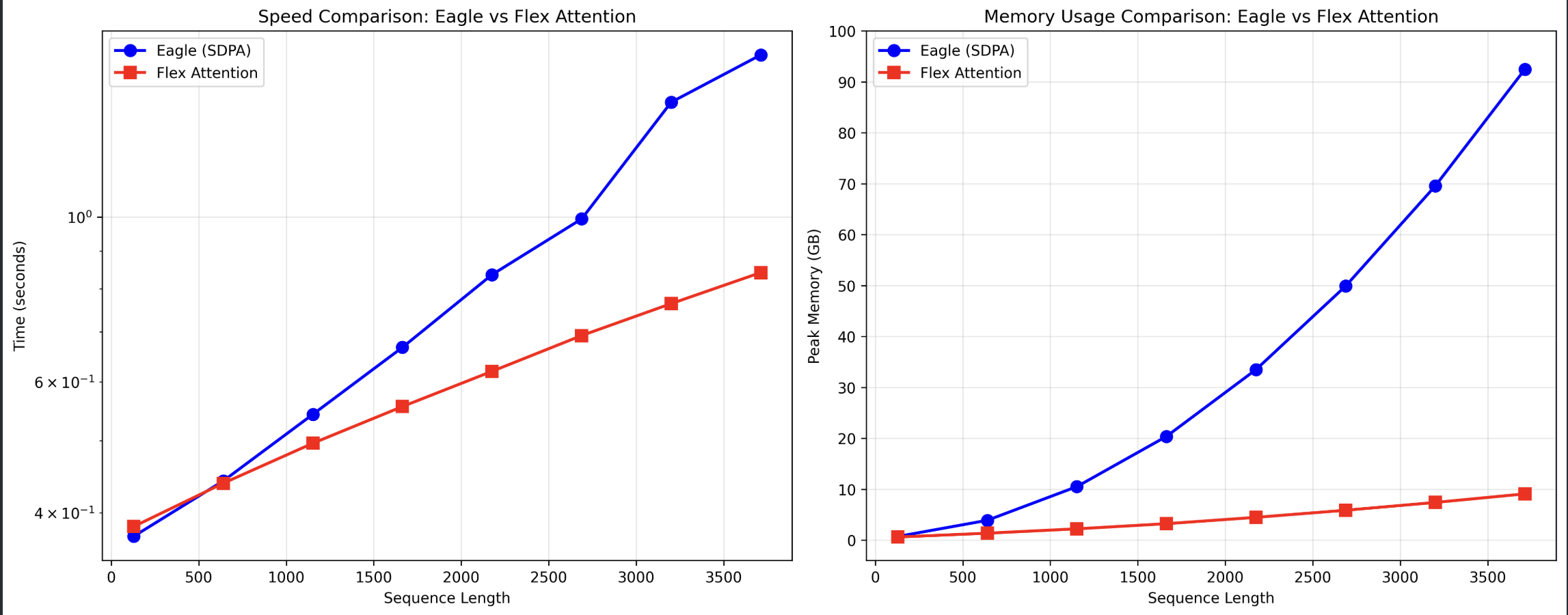
• Add Flex attention backend, uses 10~20x less memory in long context training #97
• Optimize loss calculation with in-place gradients calculation ~40% memory save #185

With the above optimizations, we have successfully trained EAGLE3 draft models for a series of open source models such as Qwen3-30B-A3B, Qwen3-235B-A22B, Qwen3-14B with 16K length context with our own created blend dataset.

EAGLE3 Training

EAGLE3 training is similar to SFT distillation training, where the prompt is masked from the loss calculation. Target model is used to generate the target probability distribution for each token. However, it is a bit different from regular distillation SFT due to the TTT mechanism: EAGLE3’s draft token generation is based the previously drafted token(actually it’s the auxiliary hidden states from the previous draft step) and the current token embedding. To make the draft model learn to generate the token in this fashion, Training-Time Test (TTT) mechanism is introduced. During training, draft model will run forward pass N times. For each step, the last hidden states from the draft model are used as the query for the next step. For each step, we calculate a loss for the new input sequence. Then towards the end, we calculate the weighted sum of the losses and backpropagate the gradient through the draft model. Due to the multiple steps of TTT, the memory footprint is significantly higher than the traditional SFT distillation training.

Another reason why memory has been an issue for EAGLE3 is for the first draft step of TTT, we need to collect 3 decoder layers’(low, mid, high) output hidden states generated from the target model and combine them with the token embeddings of the training input. These hidden states can be generated either online/on-demand or offline where all hidden states are stored in a storage. SpecForge supports both online and offline training modes. However, offline training requires storing 3 * (batch_size * seq_len) * hidden_size of bfloat16 tensor. So for Qwen3-30B-A3B with 16K context length of batch_size 1, it will be 3 * 1 * 16384 * 2048 * 2 bytes = 201326592 bytes, and that is 201 MB alone for 1 entry. We have around 50k data. That is around 10 TB of storage needed! Also, we need to count in the overhead of reading data from FileSystem -> CPU -> GPU. Thus, online training is a more reasonable choice for us. Under this setting, target model coexists with the draft model during training, reducing the memory capacity that can be used for the draft model training itself.

:::info Please notice, even if each TTT step only generates a hidden state, we are referring it as “new tokens” for the purpose of easy understanding. The diagram below illustrates the TTT mechanism. :::

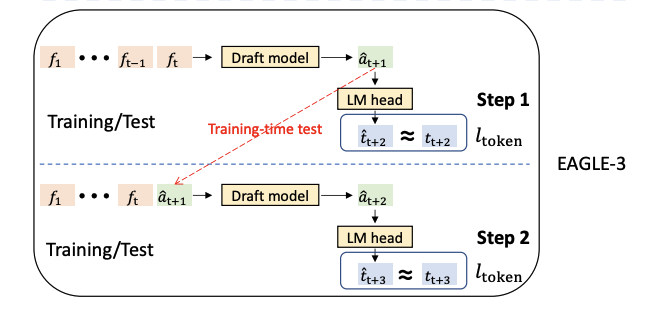
The process can be described using pseudocode as below:

hidden_states = target_model(input_ids)
input_emb = target_model.input_embedding(input_ids)
losses = []
for ttt_step in range(N):
    hidden_states = torch.cat((input_emb, hidden_states), dim=-1)
    step_hidden_states = draft_model_decoder(
        hidden_states=hidden_states,
        ...other_args,
    )
    hidden_states = step_hidden_states # update hidden states for the next step
    loss = compute_loss(step_hidden_states, target_probabilities)
    losses.append(loss)
    if not last_step:
        input_emb.shift_left(1)
        loss_mask.shift_left(1)
final_loss = weighted_sum(losses) / N
final_loss.backward()

The TTT mechanism requires a sparse attention calculation. The new “tokens” should attend to all the previous tokens. Thus, KV cache needs to be stored to keep track of the tokens from previous steps.

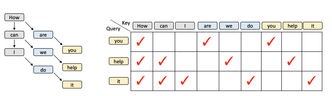
The idea in the original EAGLE3 paper is to calculate an attention weights for the first causal part and the following sparse part separately and then run softmax. Recall that:

attention(Q, K, V) = softmax(QK^T / sqrt(d_k)) V

and the attention weights can be calculated as:

weights = QK^T / sqrt(d_k)

For the first part, the attention can be calculated with:

attn_weights = query_states @ k.transpose(2, 3) / math.sqrt(head_dim)

The rest can be calculated with:

for i in range(kv_cache_length):
    ki = kv_cache[i]
    # dot product between query and key
    attn_weightsi = (qi * ki).sum(-1) / math.sqrt(head_dim)
    # concatenate the attention weights
    attn_weights = torch.cat((attn_weights, attn_weightsi), dim=-1)

attn_weights = nn.functional.softmax(attn_weights, dim=-1, dtype=torch.float32).to(query_states.dtype)
attn_output = torch.matmul(attn_weights0, v0)
for i in range(1, lck):
    vi = cache_v[i]
    attn_weightsi = attn_weights[..., q_len + i - 1]
    attn_outputi = attn_weightsi[..., None] * vi
    attn_output = attn_output + attn_outputi

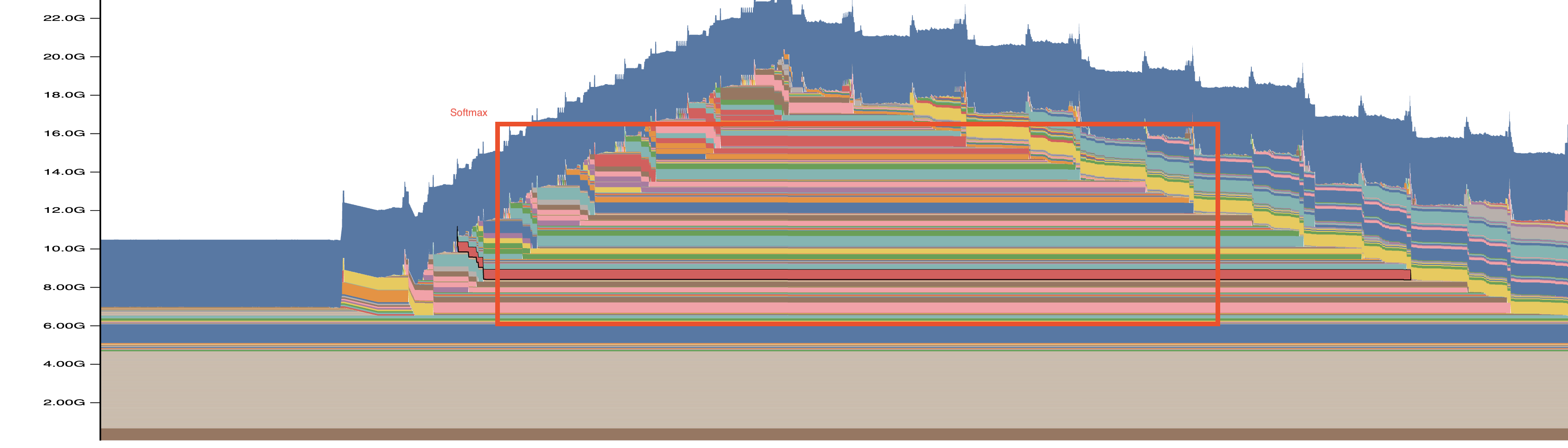
This sounds good as it reduces the amount of calculation needed. However, this approach uses naive softmax calculation which stores the entire attention weights after softmax Sij = Q_i * K_j^T / sqrt(d_k) as activations(O(n^2)) in memory unlike Flash Attention’s online softmax. According to memory profiling, we can see memory usage spike accordingly:

Flex Attention

Flex attention is a project from pytorch team. The core idea is to leverage torch inductor to compile a simple python function into a hand-written highly efficient attention kernel implemented in triton. It is extremely useful for sparse attention calculation due to its mechanism to skip blocks that does not require calculation. FlexAttention implements a BlockMask data structure which efficiently precomputes which blocks along a dimension can be skipped. Besides, it also devides the rest of the blocks into partial blocks and full blocks. Full blocks can skip the mask_mod operation, which makes it a little bit faster with less operations. Most importantly, the generated kernel uses online softmax to save memory, which fits our need here. It also supports broadcasting on batch dimension and supports Grouped Query Attention (GQA). Thus, our job become simple: construct a BlockMask based on the TTT mechanism described above and let Flex Attention handle the rest.

We build eagle BlockMask as below:

def causal_mask(b, h, q_idx, kv_idx):
    # Causal will keep shrinking by 1 diagnol due to appended suffix
    # Shirnk the causal by diagnol
    causal_mask = q_idx - shift_left >= kv_idx
    padding_mask = kv_idx < seq_lengths[b]
    return causal_mask & padding_mask

def suffix_mask(b, h, q_idx, kv_idx):
    suffix_mask = kv_idx >= Q_LEN
    padding_mask = kv_idx % Q_LEN < seq_lengths[b]
    diagnol_mask = (kv_idx - q_idx) % Q_LEN == 0
    return suffix_mask & padding_mask & diagnol_mask

mask_mod = or_masks(causal_mask, suffix_mask)

Then we pass the maskmod when creating block mask and pass the created block mask into flex attention.

block_mask = create_block_mask_func(
    mask_mod=generate_eagle3_mask(
        seq_lengths=seq_lengths,
        Q_LEN=q_len,
        KV_LEN=key_cache.shape[-2],
        shift_left=lck,
    ),
    B=bsz,
    H=1,  # Rely on broadcast
    Q_LEN=q_len,
    KV_LEN=key_cache.shape[-2],
    device=query_states.device,
)

attn_output = flex_attention(
    query=query_states,
    key=key_cache.contiguous(),
    value=value_cache.contiguous(),
    block_mask=block_mask,
    enable_gqa=True,
)

You might notice that we need to pass in KV cache. We leveraged DynamicCache class defined in transformers libarary provided by huggingface to store the KV cache.

Sounds simple, right? However, during the benchmarking, we did not see much memory reduction or speedup. In some cases, the memory usage even increased. After some investigation, we found out we need torch.compile() to leverage the compiled triton kernel. However, after enabling torch.compile(dynamic=True), the outputs of the flex attention does not match the naive implementation as the input shape can change due to different length each batch. I tried a few things such as using padding to multiple of 256 and leverage StaticCache to fix the shape. However, StaticCache can not be used for backward propagation as the one big tensor allocated will be modified multiple times during the backward pass, which is not allowed. Things seem to be stuck.

Things took a turn when pyTorch team release torch2.8. After upgrading to torch2.8. The kernel compiled handles dynamic shapes correctly.

Another lesson learned is that when we write test to compare naive attention with flash-attention style attention mechanism, we should avoid using torch.randn() as it does not cap on the range of the values. This can lead to overflow causing precision tests to fail.

After the integration, we can see great memory reduction and speedup during the training:

In-place Gradient Calculation

After Flex Attention optimization, the bottleneck now shifts to the loss calculation phase. EAGLE3 training calculates the soft target probabilities loss for each TTT step. The loss calculation is done as below:

@torch.compile(dynamic=None)
def _compute_loss(logits, target_p, position_mask):
    logits = logits.float()
    out_logp = nn.LogSoftmax(dim=2)(logits)
    plogp = target_p * out_logp
    loss = -torch.sum(position_mask * plogp, 2).mean()
    return loss

See the memory profiling below. The memory peak is the TTT steps of loss calculation’s gradients and intermediate tensors for backward pass.

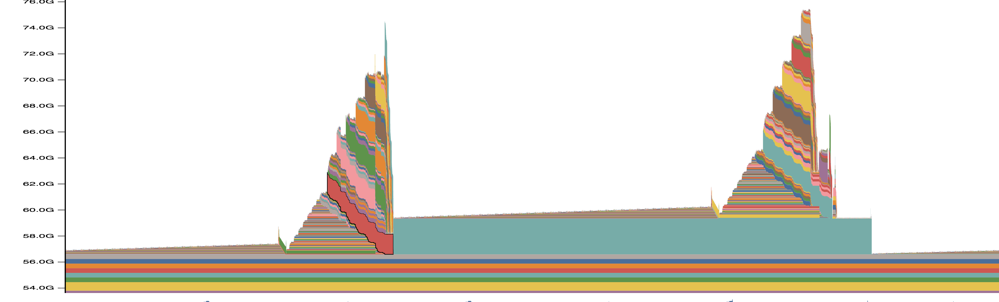
Thus, the second improvement we made is to optimize the loss calculation with in-place gradient calculation. This is a trick to leverage the input logits’ tensor to store the gradients during the backward pass. This can roughly save half of the memory since gradients are of the same shape as the logits. This technique is used for cross entropy kernel in Liger Kernel repo. However, we can’t directly leverage the library for the following reason:

1. Liger-Kernel only handles one hot encoding cross entropy loss. In SpecForge, the loss is calcuated with soft target probabilities. Due to this, the gradients calculation needs to be separated into another kernel, where Liger fuses forward and backward pass into one kernel.
2. Liger-Kernel applies kernel replacement through monkey patching. Here, we don’t have a module. Instead, we create a new LogSoftmaxLoss class that extends torch.autograd.Function and use it directly.

The pseudocode of the triton kernel is as below:

class LogSoftmaxLoss(torch.autograd.Function):

    @staticmethod
    def forward(ctx, logits, target_p, position_mask):
        loss = torch.zeros((B * T, 1), device=logits.device)
        m = torch.zeros((B * T,), device=logits.device, dtype=torch.float32)
        d = torch.zeros((B * T,), device=logits.device, dtype=torch.float32)
        log_softmax_forward_kernel[grid](
            logits,
            target_p,
            position_mask,
            m,
            d,
        )
        ctx.save_for_backward(logits.detach(), target_p, position_mask, m, d) # Detach here is the key to avoid duplicate the memory.
        return loss.mean()

    @staticmethod
    def backward(ctx, grad_output):
        logits, target_p, position_mask, m, d = ctx.saved_tensors
        log_softmax_backward_kernel[grid](
            logits,
            target_p,
            position_mask,
            m,
            d,
        )
        return logits, None, None

And in the kernel, we will calculate the loss using online softmax and store row-wise m and d.

@triton.jit
def log_softmax_forward_kernel(...):
    # first pass to calculate m and d
    for i in range(0, n_cols, BLOCK_SIZE):
        logits = load_logits
        block_max = tl.max(tl.where(mask, logits, float("-inf")))
        m_new = tl.maximum(m, block_max)
        d = d * tl.exp(m - m_new) + tl.sum(
            tl.where(mask, tl.exp(logits - m_new), 0.0)
        )
        m = m_new

    loss = 0.0
    # second pass to calculate the loss
    for i in range(0, n_cols, BLOCK_SIZE):
        logits = load_logits
        target = load_target
        # log-softmax: log(exp(x - max) / sum) = (x - max) - log(sum)
        normalized_logits = logits - m
        log_normalizer = log(d)
        log_softmax_logits = normalized_logits - log_normalizer
        weighted_log_prob = target * log_softmax_logits
        loss += sum_reduce(weighted_log_prob)
    tl.store(loss_ptr, -loss)
    tl.store(m_ptr, m.to(tl.float32))
    tl.store(d_ptr, d.to(tl.float32))


@triton.jit
def log_softmax_backward_kernel(logits_ptr, ...):
    # First pass: compute sum of (target * grad_output)
    for i in range(0, n_cols, BLOCK_SIZE):
        target = load_target
        target_grad_sum += sum_reduce(target * grad_output)

    # Second pass: compute log-softmax gradients
    for i in range(0, n_cols, BLOCK_SIZE):
        logits = load_logits
        target = load_target
        softmax_prob = exp(logits - m) / d
        normalized_grad = softmax_prob * target_grad_sum
        grad = -(target * grad_output - normalized_grad)
        tl.store(logits_ptr, grad.to(tl.float32))

Here is the benchmark results of the peak memory reduction:

Config (B, T, V)	PyTorch (ms)	Triton (ms)	Speedup	PyTorch Mem (GB)	Triton Mem (GB)	Memory Save
(1, 1024, 32000)	449.08	435.22	1.03x	1.85	0.98	46.7%
(1, 4096, 32000)	127.67	7.03	18.15x	7.32	5.62	23.3%
(1, 4096, 64000)	20.78	24.35	0.85x	14.65	11.23	23.3%
(1, 8192, 32000)	20.48	13.56	1.51x	21.48	14.65	31.8%
(1, 8192, 64000)	41.14	48.11	0.86x	29.30	22.46	23.3%
(1, 16384, 32000)	41.11	26.95	1.53x	42.97	29.30	31.8%