Dynamic Speculative Decoding

In the previous post, I covered the training techniques and optimizations regarding to EAGLE3 speculative decoding. We are able to create a fairly good draft model ready to be served. Thus, the question is: How effective is speculative decoding in practice? What are the scenarios where speculative decoding can be beneficial? How do we tune our serving configurations to get the best performance?

This post will cover explorations and discussions from my LinkedIn work. We propose a dynamic speculative decoding approach to enable the best performance under different scenarios.

Problem Context

At LinkedIn, we used a series of LLM models as assistants such as Sales Assistant, Hiring Assistant, etc. Thinking and reasoning was often needed for these use cases. In practice, each request would have around 1000 tokens prompt and generate around 600 tokens response. The cache hit rate was around 15% for these use cases. The analysis in the following section heavily relies on these assumptions.

What matters for speculative decoding?

The overall effectiveness of speculative decoding accelearation is determined by the following factors:

1. The acceptance rate of the proposed tokens. This depends on the alignment between the draft model and the target model.
2. The ratio of the per forward pass time between the target model and the draft model. The higher the ratio, the more beneficial speculative decoding is. Thus, speculative decoding works better for larger models.
3. The batch size and input context length. Speculative decoding is more beneficial for smaller batch sizes and shorter context lengths. Thus, it is more helpful in agentic, reasoning user scenarios. We will focus on the analysis for the batch size as it is more related to our use cases. The context length issue can be addressed by using kv compression, hierarchical speculative decoding, etc.

Roofline Model Perspective Analysis

To recap what is speculative decoding, it is a inference speedup technique to draft multiple tokens using a draft model(usually a single decoder layer) and verify them in parallel with the target model. In essence, it can be considered as a method to enlarge the batch size to saturate computation. Here, we will explain step by step. First, let’s analyze regular decoding phase with roofline model analysis.

Firstly, a very important observation made in this paper Mind the Memory Gap: Unveiling GPU Bottlenecks in Large-Batch LLM Inference is that for smaller batch sizes, majority of the time for a decoding step is spent on the matrix multiplication operations rather than attention operations.

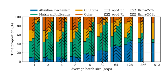
This is because we have many matrix multiplications operations in the model:

1. FFN layers with up_proj and down_proj
2. Attention layers with qkv_proj and o_proj

FFN counts about 70% of the parameters of a decoder layer while attention layer counts for the rest 30%. Even though the sequence length is very small, the matrix multiplication operations still dominate the decoding time. At small batch sizes, both matrix multiplication and attention operations are memory-bandwidth bound. The analysis are as the following:

Our theoretical maximum arithmetic intensity for a H100 GPU can be calculated as:

H100 FLOPS = 1.979e15 FLOPs/s = 1979 TFlops/s

H100 Memory Bandwidth = 3.35TB/s

1979 TFlops/s / 3.35TB/s ~= 298

Matrix Multiplication Analysis

FLOPs = B * hidden_dimension * intermediate_dimension

Memory Traffic = B * hidden_dimension + hidden_dimension * intermediate_dimension + B * intermediate_dimension

Arithmetic Intensity = FLOPs / Memory Traffic = B Flops/Byte

B = 1 for batch size = 1

Arithmetic Intensity = B = 1 Flops/Byte

Attention Analysis

Due to the nature of autoregressive generation, Q = B during the decoding phase for each query in the batch and KV cache can be 10000x larger than Q. Let’s do some simple roofline model analysis for batch size = 1 and kv cache length = 1000 for an 8B model with MHA using Flash Attention.

FLOPs = 4 * B * head_num * head_dim

Memory Traffic = 2 * B * head_num * head_dim * 2(bf16) = 4 * B * head_num * head_dim

Arithmetic Intensity = FLOPs / Memory Traffic ~= 1 Flops/Byte

As you can see, for the attention operation, even with Flash Attention, the compute power of our GPU is extremely underutilized(298x). We can use GQA or even MQA to further improve the arithmetic intensity. GQA is 298 / 8 ~= 37x, MQA is 298 / 32 ~= 10x. More importantly, the arithmetic intensity does not depend on the batch size or the context length!

When speculative decoding shines?

As we can see, both attention and matrix multiplication operations are memory-bandwidth bound at small batch size. Our context length is 1000, which is « hidden_size(4096) « intermediate_size(14336). As a result, attention operation will take way less time than matrix multiplication as it moves less data from HBM to SRAM. Based on this, we can have the following reasoning:

For decoding phase at small batch size:

1. Latency is dominated by matrix multiplication.
2. Matrix multiplication arithmetic intensity scales with B(batch size).
3. B is small compared to hidden_size and intermediate_size.
4. As a result, we can increase the batch size until we saturate the computation with a higher arithmetic intensity.

Given we are roughly at B Flops/Byte for attention operation, we can theoretically increase the batch size to 298 without sacrificing the latency. This is where speculative decoding comes into play.

For a regular decoding, the arithmetic intensity is independent of the batch size. However, speculative decoding solely increases the batch size without increasing the memory traffic as the KV cache is shared for a single request. As a result, we can times the arithmetic intensity by N times, where N equals to the number of proposed tokens.

Arithmetic Intensity = FLOPs / Memory Traffic * Number of proposed tokens = B * N Flops/Byte

Now let’s calculate the speed up effect for small batch size scenario. Let’s assume our average accept length for each step is 3 tokens with 16 tokens proposed for each step. Now our theoretical speed up for decoding is:

T(reg) = regular decode time per step

T(verify) = target verify time per step

T(draft) = draft time per step

Speed up = 3 * T(reg) / (T(verify) + T(draft))

Again, quoting from the paper Mind the Memory Gap: Unveiling GPU Bottlenecks in Large-Batch LLM Inference:

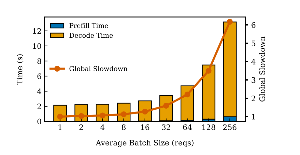
We can see that the slowdown is almost linear with the batch size at small batch size. This is because at memory-bandwidth bound, small batches are far from saturating the 3.35TB/s memory bandwidth. Thus, the increase in batch size do not increase the latency by much. It would take ~400 batch size to saturate the memory bandwidth completely.

T(ver) = 1.5 x T(reg), and T(draft) ~= 1/20 x T(reg)

Speed up ~= 3 / 1.5 = 2

We roughly get a 2x speed up for speculative decoding at batch size = 1, number of proposed tokens = 16. In practice, we don’t have as much improvement due to factors like CPU overheads, synchronization overheads, etc. Also, tree mask attention is not very easy to optimize compared to causal attention.

When does speculative decoding loose its magic?

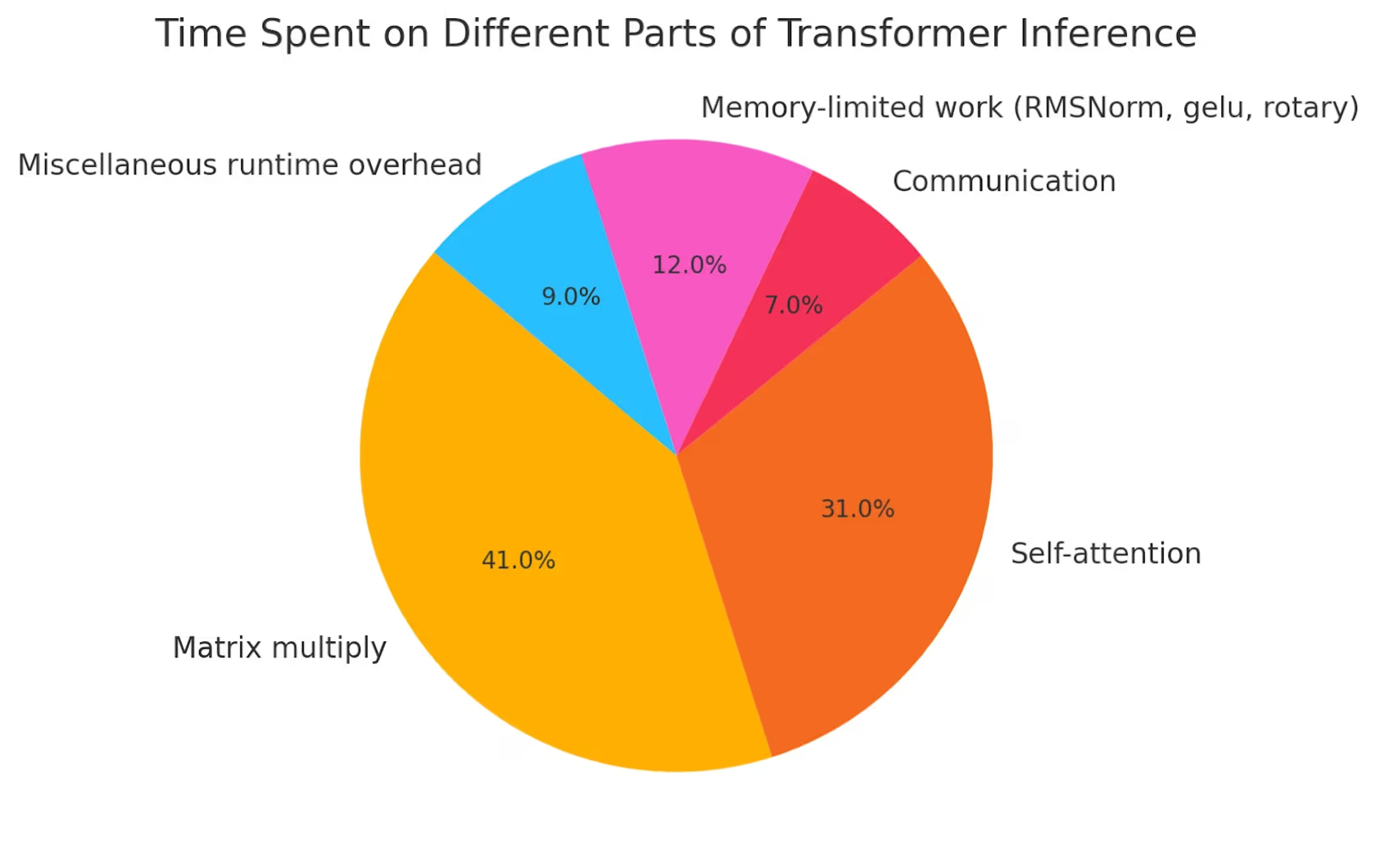
Now let’s change the scenario to a larger batch size. According to a research done by augment code, at larger batch size like 2048 with context length 8192, the model latency almost evenly split between attention and matrix multiplication. In our case, we have 8x less context length but also 8x smaller batch size. However, this batch size still enough to shift our matrix multiplications into computation bound. Under this scenario, more batch size introduced by speculative decoding will result in longer latency for the matrix multiplication part. And for the attention opeartion, because the runtime complexity is O(n^2), the latency will scale quadratically with the input sequence length. As a result, the speculative decoding will not be beneficial for larger batch size.

At this stage, our total runtime will increase linearly with the batch size. Given the same acceptance length, the speed up will be:

T(ver) = 16 x T(reg), and T(draft) ~= 1/20 x T(reg)

Speed up ~= 3 / 16 ~= 0.1875

We are not getting worse inference speed without getting higher throughput.

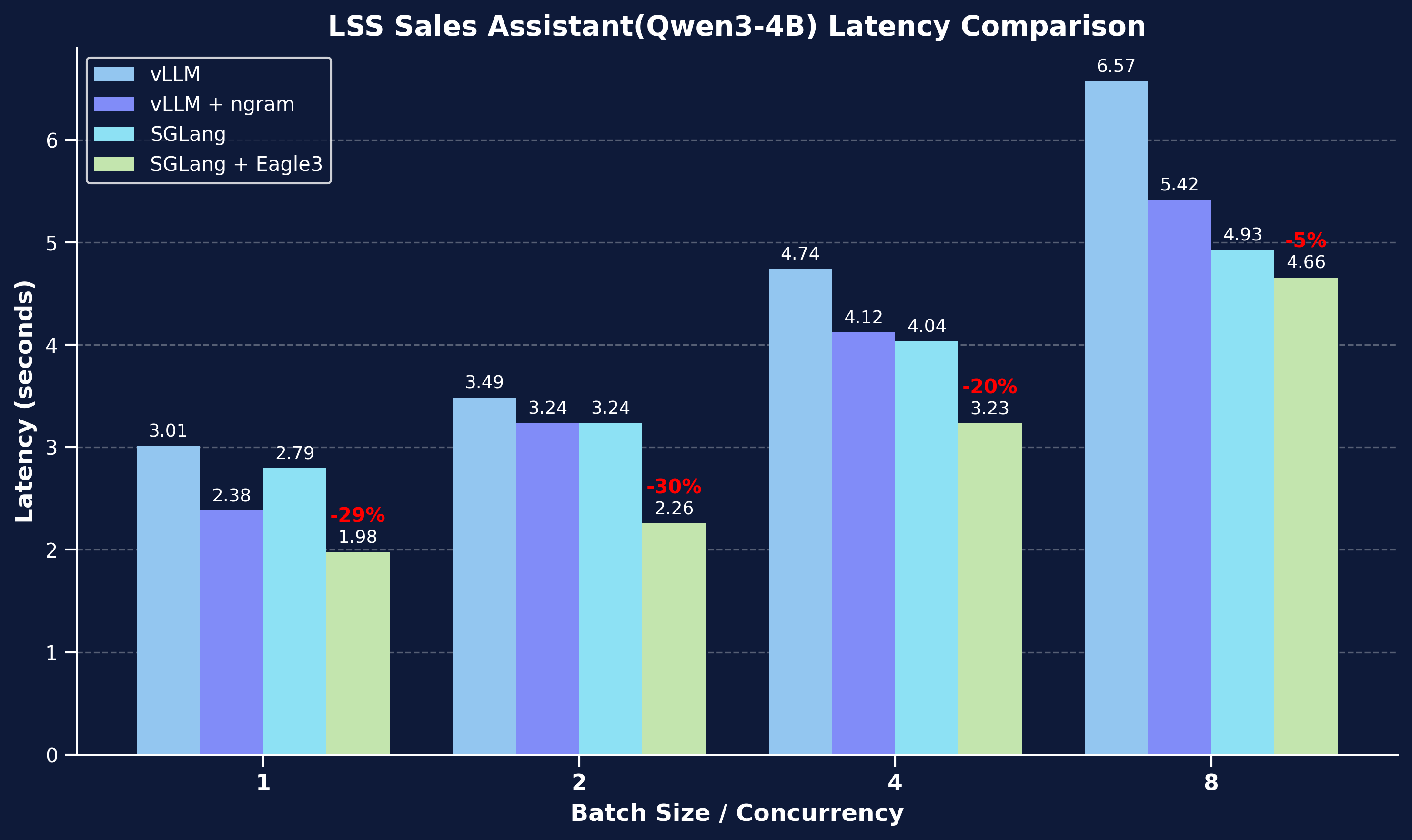
Here is the benchmark result for speculative decoding with 32 proposed tokensat different concurrency levels for a Qwen3-4B model. We lost speed up at batch size = 16. This is because we are at equivalently 32 * 16 = 512 batch size. This is already at computation bound and the latency increase per step cancels out the multiple tokens accepted. We compare between vLLM baseline, SGLang baseline, vLLM ngram and SGLang EAGLE3.

Dynamic Speculative Decoding

As we can see, speculative decoding is only beneficial for small batch size and short context length. For larger batch size, speculative decoding will not be beneficial. Thus, we propose a dynamic way to adjust the number of proposed tokens based on the in-flight batch size or even turn off speculative decoding completely given a pre-determined threshold.

First, let’s discuss the user scenario of speculative decoding. For most of the inference providers, they don’t need dynamically adjust the config for individual serving instances. This is because there is a almost always a requirement on SLA on latency. They can benchmark the best batch size to generate the best throughput without violating the fixed latency SLA. They can also adjust on a cluster level on how many machines to allocate to keep the batch size relatively stable for each instance. However, our use case is more resource-limited. Give that we have x GPUs available for the expected traffic. We want to minimize the latency for different QPS scenarios and we don’t have the luxury to scale up and down.

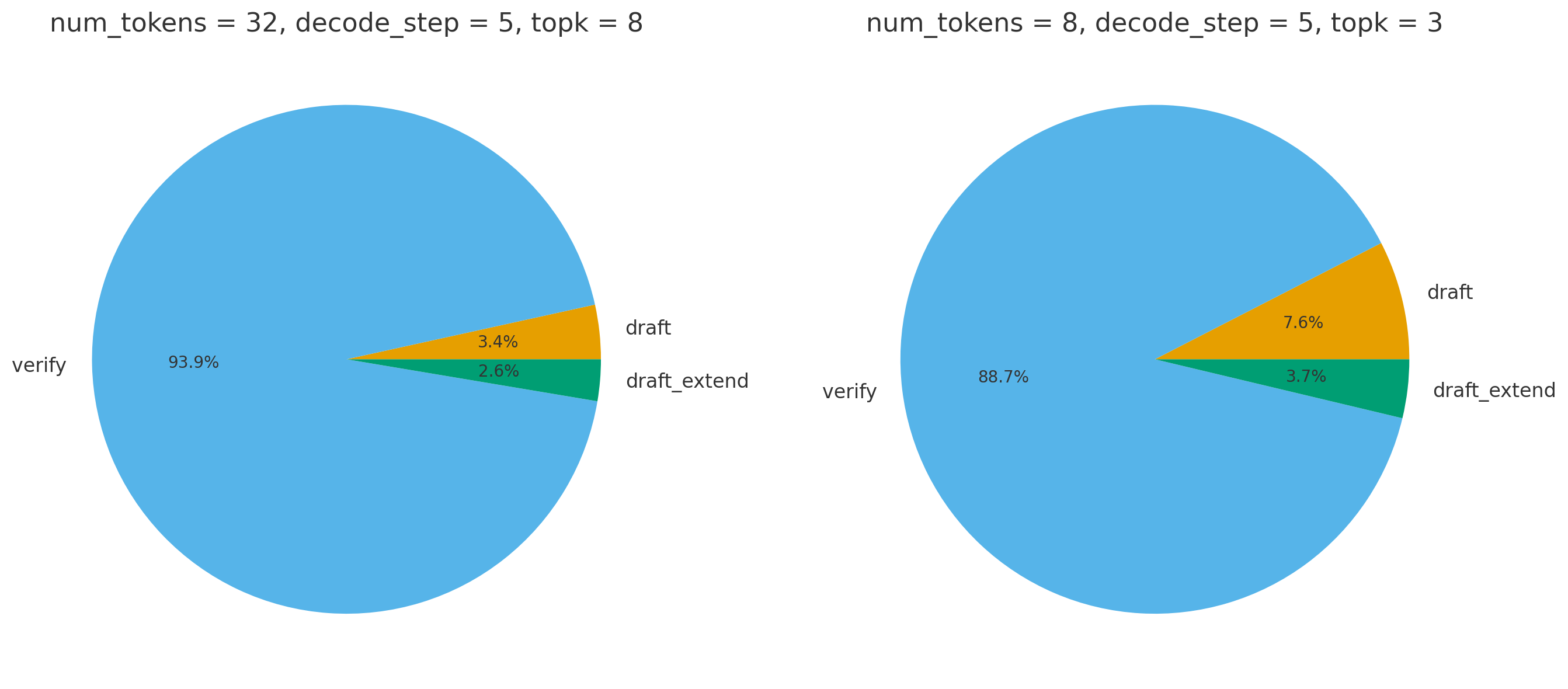
To design an effective dynamic speculative decoding strategy, we first need to understand the time breakdown of the inference time of a round-trip of a decode step. We measured the time for multiple different batch sizes and determined that: the draft phase and draft extend phase takes up only 1% of the time, the rest is spent on the target verify. We also found that the prefill time can be ignored since it is around 1% of the end to end latency.

Benchmark Table

Config	Accept Length	Target Prefill (ms)	Draft Prefill (ms)	Decode Total (ms)	E2E Latency (ms)
baseline	0.00	20.25	N/A	3651.19	3671.44
5, 3, 8	2.55	20.10	2.67	2287.52	2874.65
5, 8, 32	3.10	19.91	2.62	3188.71	3486.09

*Config is: [speculative_num_steps, speculative_topk, speculative_num_draft_tokens]

Our Solution

We have implemented a dynamic speculative decoding strategy on top of SGLang EAGLE3. There are two scenarios we want to cover:

1. Dynamically adjust the number of proposed tokens for verification.
2. Turn off speculative decoding completely given a pre-determined threshold.

Dynamic SpecDecode Config

We have noticed that topk branching in draft tree has less impact on the average acceptance length. Besides, our benchmark indicates that the number of draft steps has a relatively small impact on the overall latency. In addition, because a lot of kernel operations can not be easily adoptive to the number of draft steps. e.g. tree attention mask generation, kv cache allocation, etc. Here is the measured time span in each stage during EAGLE3 speculative decoding.

Turning off Spec Decode

We pre-determine a batch size when spec decode does not provide any speed up through benchmarking. Turning off spec decode means target model runs regular decode step by step.

Implementation Details

Dynamically changing the topk in the draft tree is relatively easy because most of the kernel operations are not affected by the number of topk. Turning off spec decode needs more careful treatment because of continuous batching. We need to treat entering from spec decode to regular decode and from regular decode to spec decode differently. Besides, we need to run an additinoal “draft extend” step after target regular decode to keep the kv cache consistent for generations when spec decode is turned back on. The process can be summarized in the following diagram:

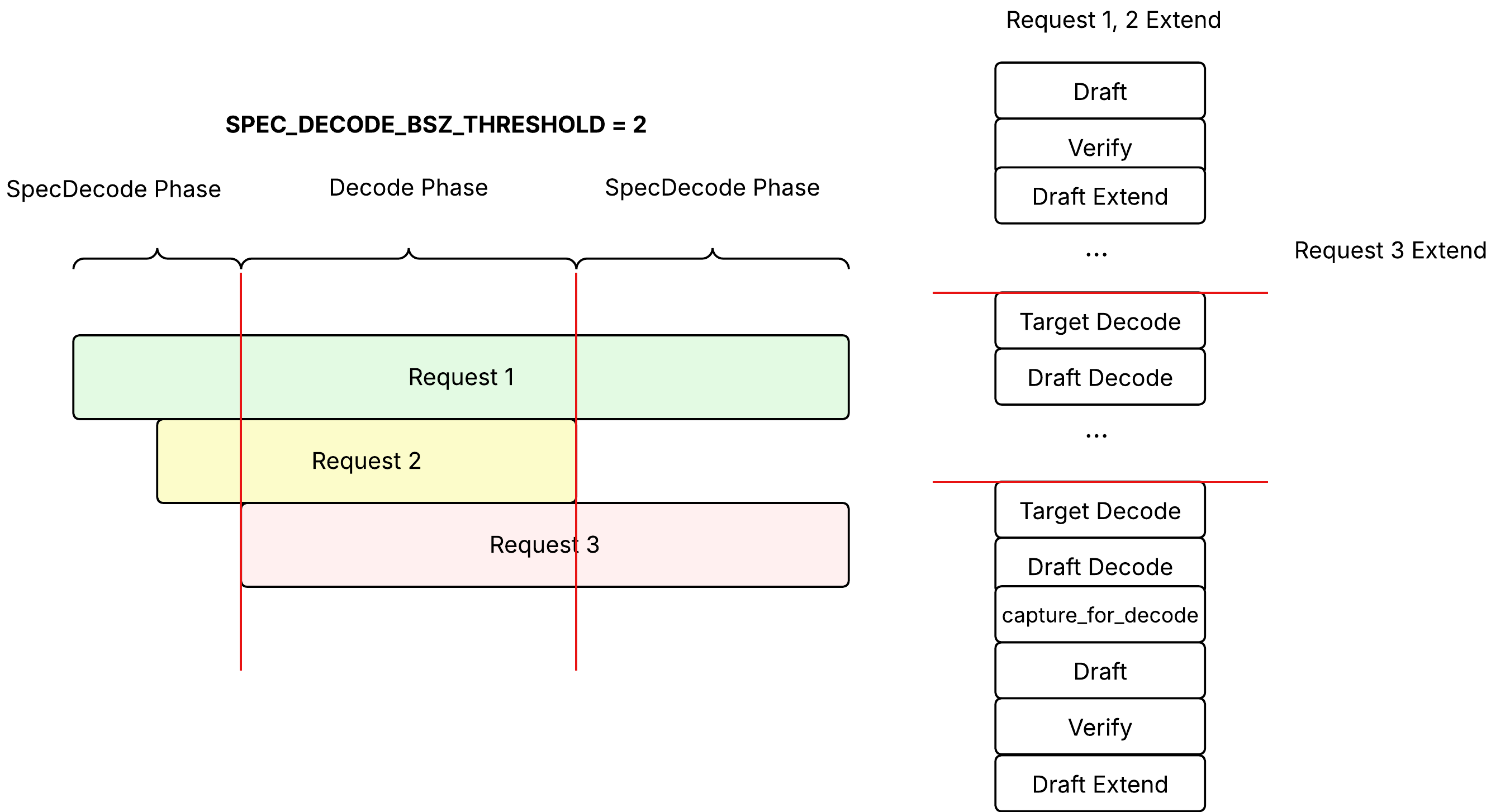
In the SGLang batch scheduler, we determine the current batch size after merging with prefill batch and filtering out finished requests. After the batch size is determined, we decide whether to run spec decode or regular decode based on the server arguments SGLANG_SPEC_DECODE_BATCH_SIZE_THRESHOLD. If the batch size is less or equal to the threshold, we run spec decode. Otherwise, we run regular decode.

def update_running_batch(batch: ScheduledBatch):
    batch.filter_batch()
    # Update speculative decoding enablement flag for the current batch
    if not self.spec_algorithm.is_none() and batch is not None:
        threshold = envs.SGLANG_SPEC_DECODE_BATCH_SIZE_THRESHOLD.get()
        previous_enabled = batch.is_spec_enabled_for_batch
        batch.is_spec_enabled_for_batch = threshold is None or batch.batch_size() <= threshold
        if previous_enabled and not batch.is_spec_enabled_for_batch:
            batch.turning_off_specdecode = True
        if not previous_enabled and batch.is_spec_enabled_for_batch:
            batch.turning_on_specdecode = True

Then in EAGLE worker, we a check for decode forward mode and batch.is_spec_enabled_for_batch. If so, we run the target worker for a regular decode and pass the captured hidden states to the draft worker:

def forward_batch_generation(self, batch: ScheduleBatch) -> GenerationBatchResult:
    ...
    if batch.forward_mode.is_decode() and not batch.is_spec_enabled_for_batch:
        if batch.seq_lens_cpu is not None:
            batch.seq_lens_sum = batch.seq_lens_cpu.sum().item()
        else:
            batch.seq_lens_sum = batch.seq_lens.sum().item()
        model_worker_batch = batch.get_model_worker_batch()
        model_worker_batch.spec_info = None
        model_worker_batch.capture_hidden_mode = CaptureHiddenMode.FULL
        generation_batch_result = self.target_worker.forward_batch_generation(model_worker_batch)
        self.forward_draft_extend_after_target_decode(
            batch, generation_batch_result.logits_output.hidden_states,
        )
        return generation_batch_result

The forward_draft_extend_after_target_decode is really just another decode step using draft model.

def forward_draft_extend_after_target_decode(self, batch: ScheduledBatch, target_hidden_states: torch.Tensor) -> GenerationBatchResult:
    model_worker_batch = batch.get_model_worker_batch()
    forward_batch.target_hidden_states = target_hidden_states
    forward_batch.attn_backend = self.draft_extend_attn_backend
    logits_output, _ = self.draft_model_runner.forward(forward_batch, skip_attn_backend_init=True)

This poses a problem as this slows down the regular decode as we have to run an extra “draft extend” step. This is a tradeoff we have to take. We can potentially disable spec decode as long as there is request in the batch that is doing regular decode to avoid this extra step. However, given continuous batching, as it will turn off spec decode for most of the time. To better mitigate the slowdown, we fuse the target decode and “draft extend” step into a single CUDA Graph:

class CUDAGraphRunner:

    def _capture_graph(self, bs: int):
        with patch_model(
            self.model_runner.target_model,
            bs in self.compile_bs,
            num_tokens=bs * self.num_tokens_per_bs,
            tp_group=self.model_runner.tp_group,
        ) as forward:
            with patch_model(
                self.model_runner.model,
                bs in self.compile_bs,
                num_tokens=bs * self.num_tokens_per_bs,
                tp_group=self.model_runner.tp_group,
            ) as draft_extend:
                ...
                def forward(batch: ForwardBatch):
                    target_hidden_states = forward(batch)
                    batch.target_hidden_states = target_hidden_states
                    draft_extend(batch)

                graph, output_buffers = self.capture_one_batch_size(bs, forward)
                self.graphs[bs] = graph
                self.output_buffers[bs] = output_buffers

Then we can replay the single cuda graph for both the target decode and “draft extend” step. This has brought 10% speedup comparing to no cuda graph case.

One additional complication is in the case of changing from spec decode -> regular decode, we merged previously verfied tokens with the extend generated tokens from different requests. We need to explicitly handle this case by keeping only the last token from the previously verified tokens for the next decode step.

# CPU operations, fast
accept_length = [acc + 1 for acc in self.spec_info.accept_length_cpu]
accept_length.extend([1] * (bs - len(accept_length)))
kept_output_ids = [idx - 1 for idx in list(accumulate(accept_length))]
assert len(kept_output_ids) == bs
# Indexing
self.input_ids = self.output_ids[kept_output_ids]

Future Work

The adoptive strategy we have come up with depends on predictable user behavior. e.g prompt length, output length. It also requires extensive benchmarking to determine what spec config to use at different batch size. However, to support a truly adoptive strategy. SGLang team has proposed a Multi-Armed Bandit (MAB) strategy based on the reward signal based on number of accepted tokens and processing time from historical data. This is a more advanced strategy but never merged into the main branch and we will explore it in the future. I believe this introduces more CPU side overhead and needs to be carefully designed to overlap with GPU operations.